Section 6 - Analyzing Data Using Filtering
Introduction
For this section we will be looking at analyzing data using filtering. What is filtering, basically filtering allows us to take a set of data and easily extract a set of data we are looking for, or more correctly, allows us to hide the data we don't need.
There are two filtering techniques for which I will cover and they are: -
- AutoFilter - How to Enable
- AutoFilter - Using the AutoFilter Sort Function
- AutoFilter - Using the AutoFilter Filter Function
- Advanced Filtering - Filter on a Single Criteria
- Advanced Filtering - Filter on Multiple Criteria
- Advanced Filtering - "Copy to Another Location" and "Unique Records Only" options.
AutoFilter - How to Enable
The AutoFilter is the easier of the two filtering techniques to use. To activate it within Excel 2007 simply highlight a cell within the range you wish the AutoFilter to be applied to and go to Data > Sort & Filter > Filter.
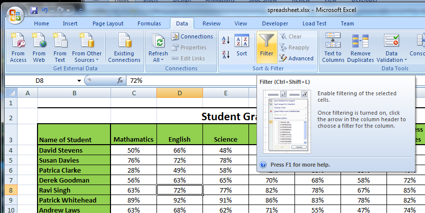
As you can see in the image below the system adds a small button with a down arrow in each cells which are the column headings. The AutoFilter itself is accessed through this down arrow.
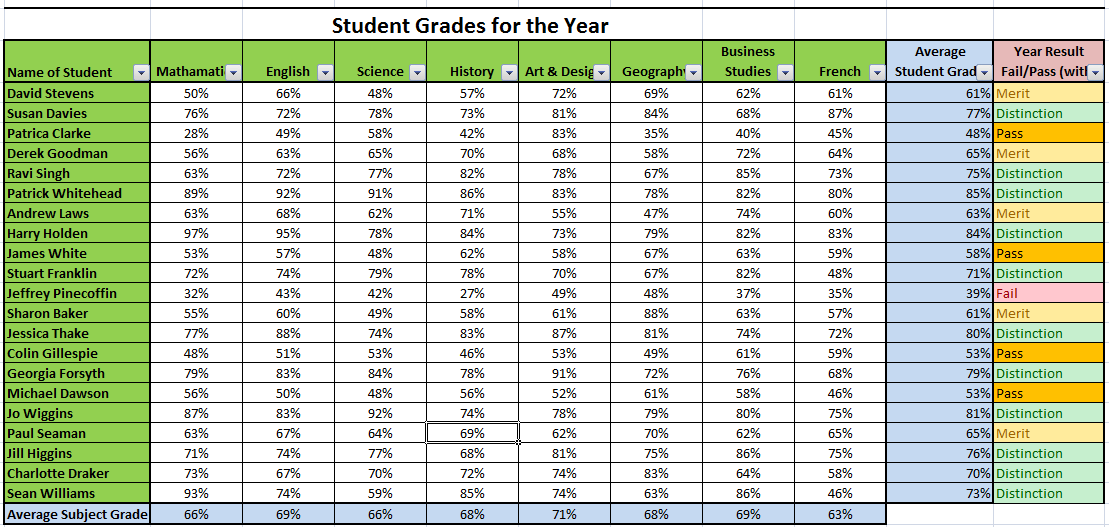
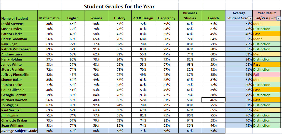
However should the system select the wrong headers for the AutoFilter you can override the system and select the specific headers which you require, to do this simply highlight the cells you wish then apply the AutoFilter as above. The image below is an example of this where only the last 2 columns have the AutoFilter applied.
 Top of Page
AutoFilter - Using the AutoFilter Sort Function
As stated before, to access the AutoFilter menu you simply need to press the small box in the lower right corner of the cell containing a column header. There are 2 types of AutoFilter menus, one of numeric data and one for alphanumeric data, however there is very little difference between the two. Pictures of these two types are below (alphanumeric on the left, numeric on the right).
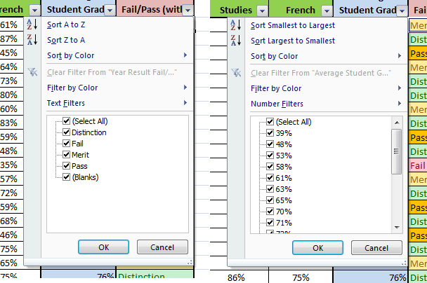
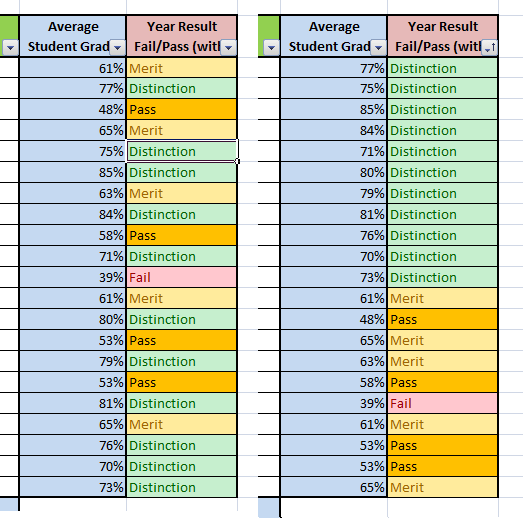
As you can see from the above image the menu is split into 3 sections. In addition to the normal Ascending and Descending sort you have the Sort by Colour option. This allows you to sort the data based on either the cell background colour or the text colour. However it should be noted that unlike the normal sorting options, the Sort by Colour option will only group the cells with the selected colours together in their relative order while the remaining cells are moved to the bottom, again retaining their relative order. The screenshot below demonstrates this.
It should be noted that the only way to reverse a sort command is to use the Undo command.
Top of PageAutoFilter - Using the AutoFilter Filter Function
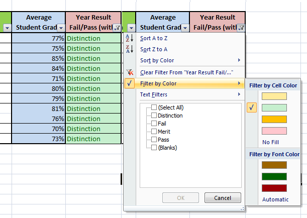
The other sections within the AutoFilter menu are the filter options themselves. Within the first section, the first option is to clear any applied filter, however unless a filter is applied this option is greyed out. The next option is the Filter by Colour which allows you to select a single cell background colour or font colour to filter from the colours present in the selected column. Once an option is selected, any row which doesn't contain the selected colour within the filtered column will be hidden from view while the filter is applied. The below example shows an example of one of the colour filters been applied.
The next option is the "custom filters", for the alphanumeric menu it is called Text Filters while in the numeric menu it is called Number Filters. These allow the user to apply a custom filter onto the table. Below is a table listing the available options.
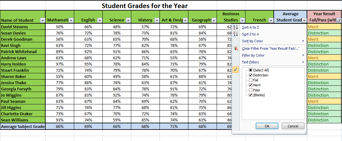
The last section contains a list of the unique data contained within the column. This section will allow you to select which data you want to display, say for example in the below example you can set up the filter to remove any students whose overall Year Result is less than Merit level.
This concludes the section relating to the AutoFilter. The next area I will look at is Advanced Filtering Techniques.
Top of PageAdvanced Filtering - Filter on a Single Criteria
Advanced filtering is another filtering function which excel provides. Advanced Filtering basically does the same job as AutoFilter, however there is a little more work required to set it up. Unlike AutoFiltering where you can input the criteria via the drop down menus in the column headers, you need to input your criteria onto the worksheet directly.
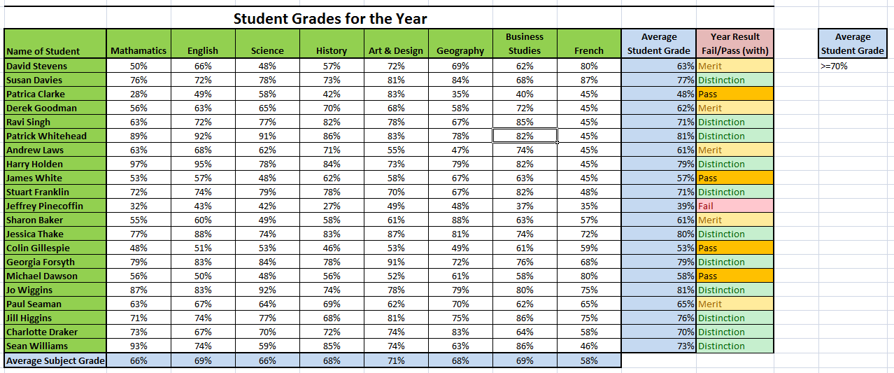
Do to this you first need to set up a new column to the side of the main workbook area. You will need to enter the column heading text exactly as it appears (formatting is ignored; the easiest way to ensure it is exact is to do a Copy and Paste command of the column header). Next you will need to input the criteria you wish to filter by in the cell directly beneath the filter column header. The below example shows how to set up the worksheet so that Excel filters to show everyone whose overall grade was greater than or equal to 70%.
Next go to Data > Sort & Filter > Advanced, this will open up a new window as shown in the below screenshot.
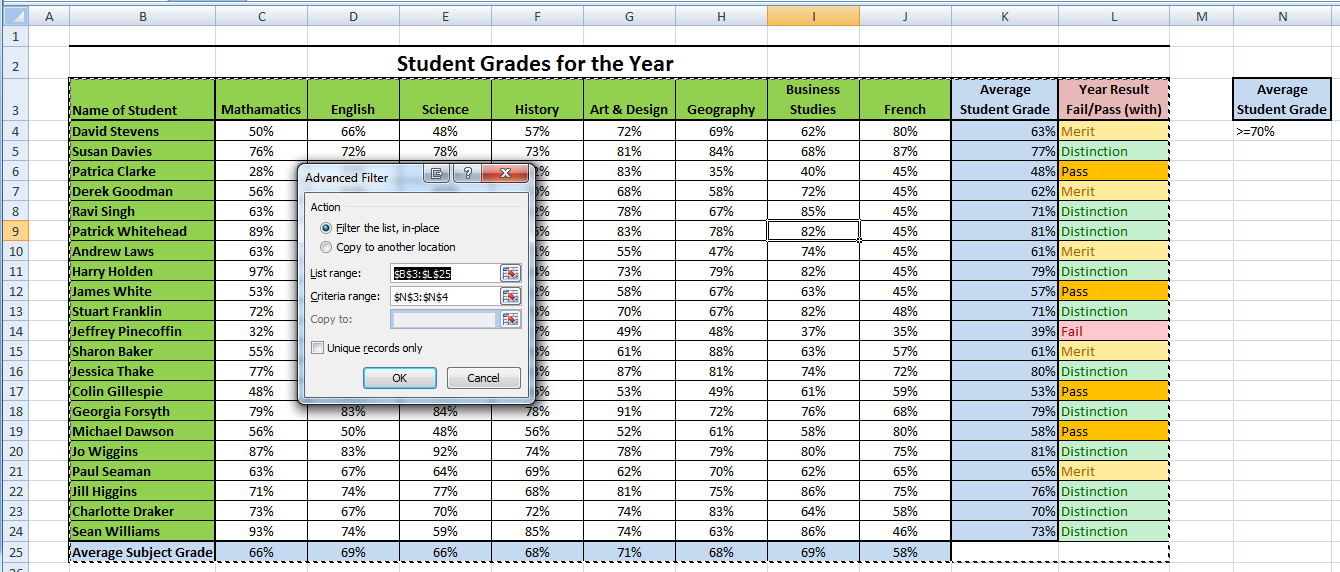
Now there are 2 options at the top called "Filter the list, in-place" and "Copy to another location", this one of the advantages which Advanced Filtering has over the AutoFilter, however the "Copy to another location" option will be covered in a different section for Advanced Filtering. The "Filter the list, in-place" option makes the Advanced Filter behave like that AutoFilter in that it will only hide the rows which contain data which don't fall into the specified criteria.
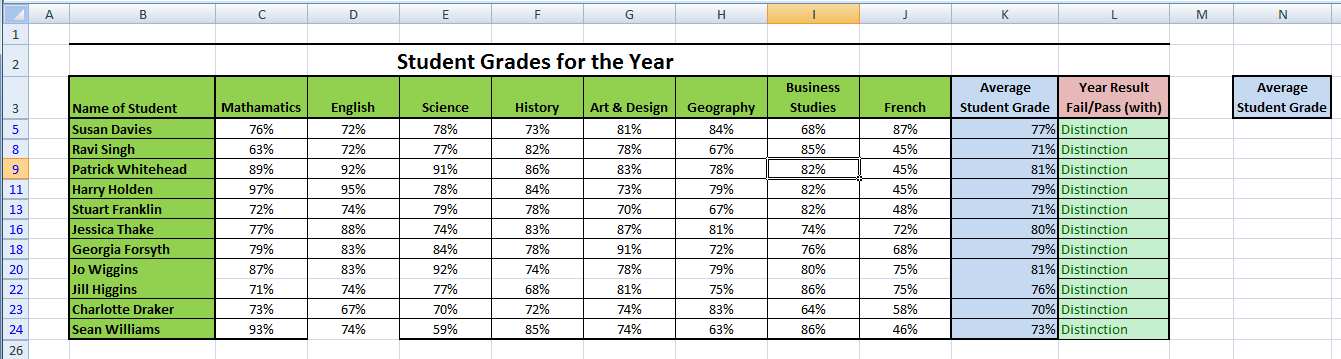
Below this we have 2 addition options, the first is the "List range:" option. This is the range you wish to filter on, Excel will select what it thinks is the data range to filter on, however you have the option to override this should you wish. The "Criteria range:" contains the addresses of the cells which contain the filtering criteria, the user simply needs to select this range. The following screenshots shows the filter been executed.
The next section will deal with filtering on multiple criteria.
Top of PageAdvanced Filtering - Filter on Multiple Criteria
The next area we will look at is filtering on multiple criteria, like filtering on a single criterion, to filter on multiple criteria you will need to add the criteria onto the workbook. However there are a couple of rules which need to be followed for the filter to work. The main rule is that each column can only have 1 criteria contained within it, as such each criteria will need its own column, again with the same heading as the column it will be filtering. The process to apply the filter is the same as before, however when selecting the criteria range you will need to include all columns which contain the criteria
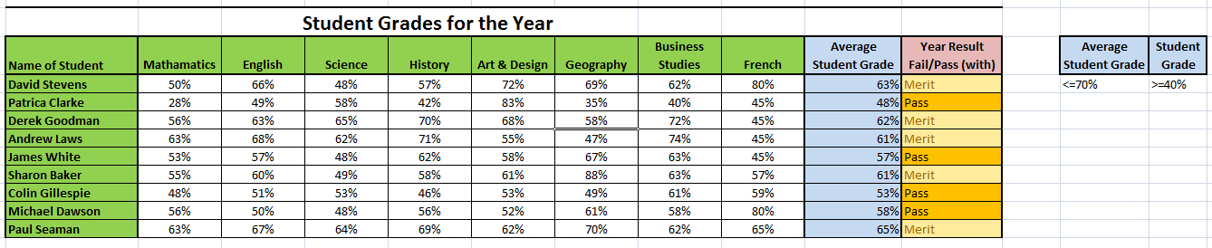
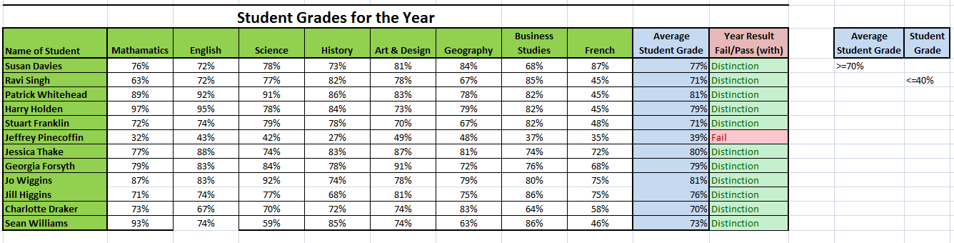
Below is a screenshot showing how to set up the worksheet to have a filter to show all Average Student Grades which are greater than or equal to 40% AND less than or equal to 70% with the filter already applied.
However the Advanced Filter isn't limited to just using AND conditions, we can use OR conditions as well. When we wish to use an OR condition we simply place the criteria on a separate row to the other criteria. The below screenshot shows a filter applied to show us all Average Student Grades which are greater than or equal to 70% OR less than or equal to 40%.
As such the normal rule for AND and OR statements is that any criteria on the same row is considered an AND statement while criteria on different rows are OR statements. However it should be noted that the criteria must be placed in the row directly below the previous criteria row when using OR criteria.
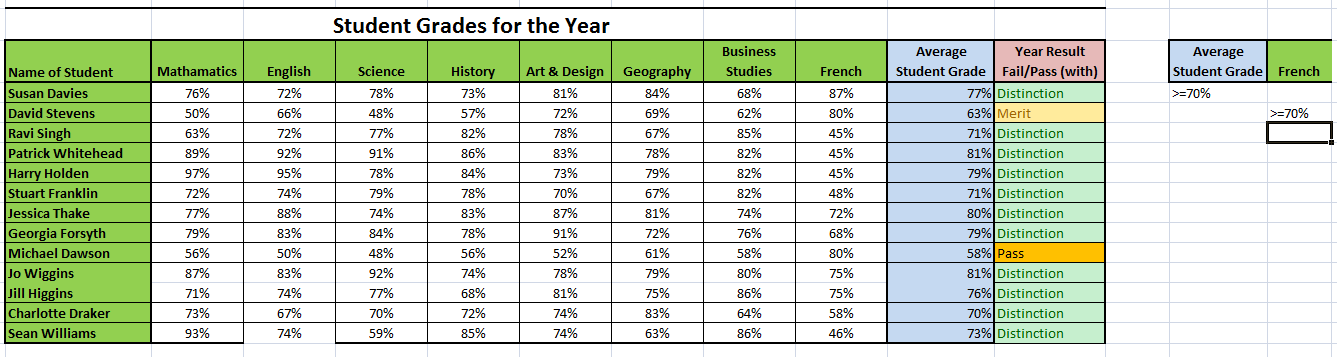
Also, like the AutoFilter the Advanced Filter can filter on multiple columns but, unlike the AutoFilter, the Advanced Filter can use OR criteria across different rows. The following screenshot shows us an applied filter to show up Average Student Grades which are greater than or equal to 70% OR French scores were greater than or equal to 40%.
The next section will cover the Copy to Another Location and Unique Records only options.
Top of PageAdvanced Filtering - "Copy to Another Location" and "Unique Records Only" options.
When using the Advanced Filter option box, there is 2 options called "Copy to another location" and "Unique Records Only". We will have a look at these options on this page.
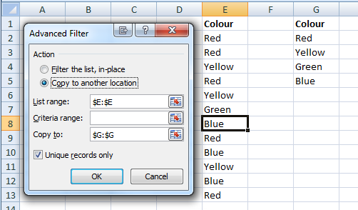
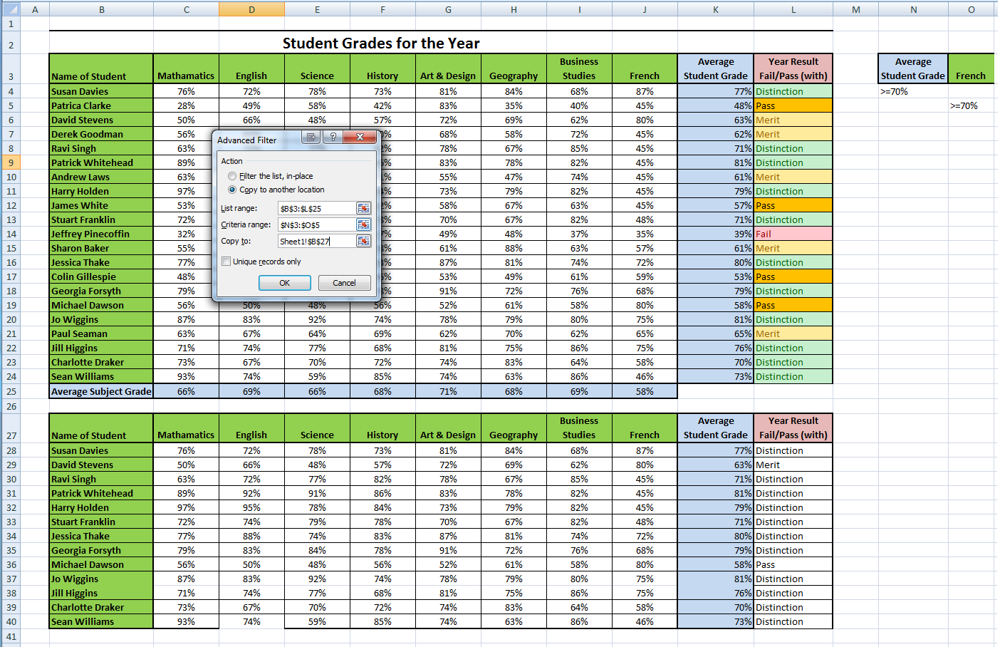
The first one we will look at is the "Copy to another location" option. Normally when a filter is applied it will only hide any rows which don't fall within the specified criteria. However this option allows us to create a copy of any data which falls within the required criteria in another part of the worksheet (the user will need to specify the location of the data in the "Copy to:" field). This has the benefit of allowing us to further manipulate the data without any risk to the original data. It should be noted however that while cell formatting is copied to the new location, any cell formulas or conditional formulas which are applied will not be. The below screenshot shows us the "Copy to another location" option been applied.
The last option is the "Unique Records Only" option. This allows the user to run a filter on, for example, a list to remove any entries which appear more than once. Again it will follow the same rules for the other options; however it must be noted that the data must have a column header for it to work properly. Below is an example on a list of peoples favourite colours with the option already applied.