Section 2 - Conditional Formatting
Conditional formatting allows the user to draw attention to cells in a spreadsheet. For example, it can be used by a company to highlight in green customers that have placed over a certain number of orders and highlight in red customers that have not placed an order for more than six months. Conditional formatting immediately highlights those customers that meet these conditions and helps the company identify customer types.
Cell Value and Specifications
In our example here, we look at a class of students and their overall marks for an academic year. It is useful for the tutor to be able to easily identify such things as which students have done well and which ones not so well. In the first instance, the tutor would like to highlight any students that did not pass particular subjects (a pass is at least 40%). She selects all the grades in the spreadsheet and chooses Home > Conditional Formatting > Highlight Cells Rules > Less Than...
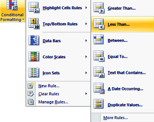
and is presented with this dialog window.
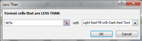
The dialog window requires a simple condition to be applied; for this example the tutor is saying display grades that are "LESS THAN 40%" and highlight those cells with "Light Red Fill with Dark Red Text". Clicking OK displays the results like this in the spreadsheet.
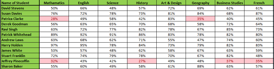
Next the tutor would like to have a look at each subject and see how many students performed above average and how many performed below average
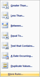
The tutor selects all the cells in the first column which contain the results for Mathematics and selects conditional formatting as before, but this time selects More rules...
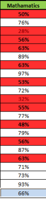
She is then presented with the following dialog window. From here she can select the type of rule that she'd like to apply. In this case she has selected Format only values that are above or below average. In the drop down box below, she selects below and then clicking the format button to the left can apply how the cells that meet this condition, will be displayed.
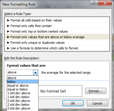
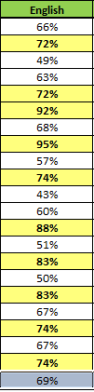
In this example the tutor has selected a red background and bold text. The same rule can be applied to show above average grades too. Here the tutor has formatted the English results to show the above average grades with a yellow background.
We have seen that conditional formatting allows the user to format their spreadsheet in ways that can draw attention to cells that meet a variety of conditions. In the example shown the tutor has been able to highlight how her students have performed over the year.
