Section 3 - Conditional Formulas
Conditional formulas allow conditions to be applied to certain cells using the IF() function. Continuing with our example of students grades for the year, the tutor wishes to find out which students failed and which ones passed the year. She knows that a fail means an average grade of less than 40% and a pass is greater than 40%. In her spreadsheet she has already set up a column titled Average Student Grade, with cells ranging from K4:K24, so she can refer to those results (cells) when setting up her IF() function.
The IF() function, follows this general specification:
IF(condition, action_on_true_outcome, action_on_false_outcome)
The tutor selects Formulas > Logical > IF
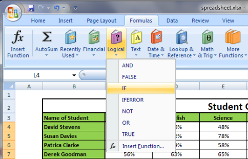
and is presented with this dialog window.
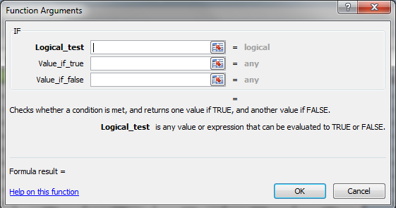
Here she is required to enter her condition; she has the choice of entering either less than 40% or greater than 40% either way the IF() function will return a true or a false value. She decides to go with less than 40% and enters the following conditions into the text boxes:
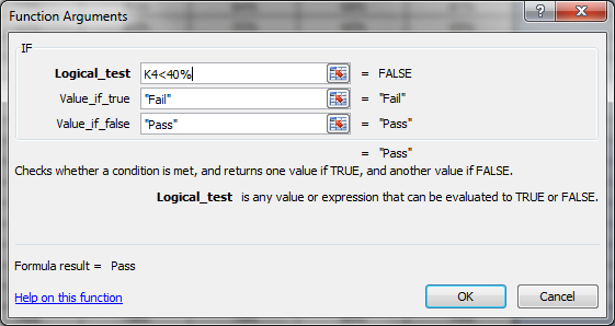
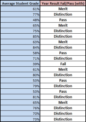
Clicking the "OK" button displays the following results:
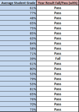
Although it is helpful for the tutor to see who passed and who failed, the previous results do not show how well those students that passed did. There are three categories of passing: Pass (between 40% and 59%), Merit (between 60% and 69%) and Distinction (70% and above).
The tutor would like to extend her IF() function to show the students that failed and those that passed in each category. Furthermore she would like to combine the IF() function with conditional formatting to highlight each category with a different colour.
The first task is to amend the function argument. The tutor can amend the function in the formulas dialog box on the main screen (see screen shot below).
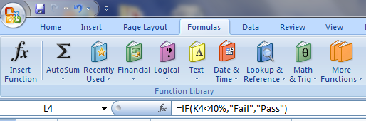
She extends the current arguments by inserting a nested IF() function. The Screen shot below show her input and reads: If the result in K4 is less than 40%, display (Fail), if the result is less than or equal to 59%, display (Pass), if the result is less than or equal to 69%, display (Merit) and if the result is greater than 70%, display (Distinction). The results are shown below.
To make these results stand out, she is now going to apply conditional formatting, to show the following:
- Fail results are highlighted in bold red text
- Pass results are highlighted in bold blue text
- Merit results are highlighted in bold black text on a yellow background
- Distinction results are highlighted in bold white text on a red background
First she selects all the cells she wishes to add a condition to and then as below selects conditional formatting > Highlight Cells Rules > More Rules > Format only cells that contain.
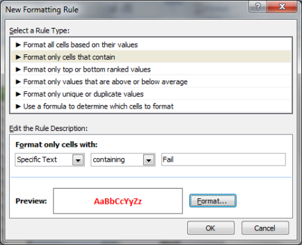
From this dialog window, she selects the conditions she wants to apply to each category in turn. The results are shown below.
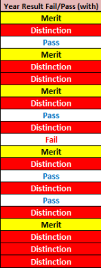
This section has shown another way of highlighting cells that meet a condition, by using conditional formulas. With the example shown, the tutor has used the IF() function to categorise students according to how well they have performed over the year.
